Statistical tests

In this session, we will introduce methods to adjust p-values to account for multiple testing, learn advanced programming techniques including for loops and writing custom functions, and cover basic statistical tests to conduct hypothesis testing for different combinations of continuous, categorical, and paired data.

Two categorical variables

There are two main tests for associations between two categorical variables: the chi-squared test and Fisher’s exact test.

Conduct these tests in R using the following functions:

chisq.test()
fisher.test()

Conduct a chi-squared test of the null hypothesis that there is no association between treatment and response versus the alternative hypothesis that there is an association between treatment and response.

library(gtsummary)

#BlackLivesMatter

chisq.test(x = trial$trt, y = trial$response)


    Pearson's Chi-squared test with Yates' continuity correction

data:  trial$trt and trial$response
X-squared = 0.22329, df = 1, p-value = 0.6365

The chi-squared test statistic is 0.22329 with associated p-value 0.6365.

Do not reject the null hypothesis since the p-value is greater than the traditional threshold for significance of 0.05.

Conduct a Fisher’s exact test (an alternative to the chi-squared test when any expected cell count is <5):

fisher.test(x = trial$trt, y = trial$response)


    Fisher's Exact Test for Count Data

data:  trial$trt and trial$response
p-value = 0.5403
alternative hypothesis: true odds ratio is not equal to 1
95 percent confidence interval:
 0.6326222 2.3394994
sample estimates:
odds ratio 
  1.213605

The p-value is 0.5403.

Do not reject the null hypothesis of no association between treatment and response since the p-value is greater than the traditional threshold for significance of 0.05.

One continuous, one categorical

The most common statistical tests for the association between a continuous and a categorical variable are the non-parametric Kruskal-Wallis test and the parametric t-test.

Conduct these tests in R using the following functions:

kruskal.test() (see also wilcox.test())
t.test()

Note that the Kruskal-Wallis test is also known as the Wilcoxon rank-sum test in the special case of a 2-level categorical variable.

“Non-parametric” means that there is no parametric distribution assumption made on the continuous variable - i.e. the continuous variable does not need to be normally distributed.

Conduct a Kruskal-Wallis test to test the null hypothesis of no association between marker status and response versus the alternative hypothesis that there is an association between marker status and response.

kruskal.test(marker ~ response, data = trial)


    Kruskal-Wallis rank sum test

data:  marker by response
Kruskal-Wallis chi-squared = 2.727, df = 1, p-value = 0.09866

Since “response” is a 2-level categorical variable, the Wilcoxon rank-sum test (without continuity correction) produces the same result:

wilcox.test(marker ~ response, correct = FALSE, data = trial)


    Wilcoxon rank sum test

data:  marker by response
W = 3043, p-value = 0.09866
alternative hypothesis: true location shift is not equal to 0

With a p-value of 0.099, do not reject the null hypothesis at the 0.05 significance level.

“Parametric” means that the test assumes a parametric distirbution - in the case of the t-test, it relies on the assumption that the continuous variable is normally distributed.

If appropriate given the distribution of the continuous variable, conduct a t-test:

t.test(marker ~ response, data = trial)


    Welch Two Sample t-test

data:  marker by response
t = -1.5851, df = 96.232, p-value = 0.1162
alternative hypothesis: true difference in means between group 0 and group 1 is not equal to 0
95 percent confidence interval:
 -0.51378857  0.05753795
sample estimates:
mean in group 0 mean in group 1 
      0.8425238       1.0706491

The p-value differs but the conclusion is the same: do not reject the null hypothesis that there is no association between marker and response.

However, in this example the data are right-skewed so a t-test is not appropriate.

library(ggplot2)

ggplot(data = trial, aes(x = marker)) +
  geom_histogram(bins = 10)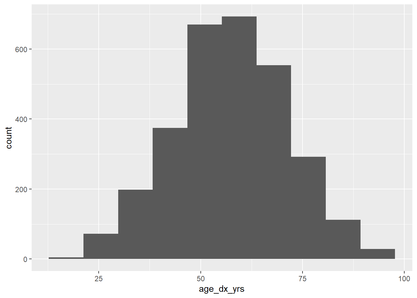

Tips:

For the preceding two tests we used the formula option to supply the information for the test
A formula in R looks like LHS ~ RHS where the left-hand side (“LHS”) is typically an outcome variable or dependent variable and the right-hand side (“RHS”) is the independent variable.
For multivariable regression, you can specify formulas in the format Y ~ X1 + X2 + X3... when there is more than one independent variable.
You must also supply the name of the dataset to the data = argument so that R knows where to look to find the specified variables.
See the help files for alternative ways to supply the information for each test

What if our categorical variables has more than 2 levels, but we want to do a parametric test? Then we will use ANOVA. ANOVA tests the null hypothesis of no association between marker and grade, which has more than two levels so a t-test is not appropriate, and relies on the assumption that the continuous variable is normally distributed.

lm_mod <- lm(marker ~ grade, data = trial)
anova(lm_mod)

Analysis of Variance Table

Response: marker
           Df  Sum Sq Mean Sq F value  Pr(>F)  
grade       2   5.385 2.69264  3.7529 0.02523 *
Residuals 187 134.168 0.71748                  
---
Signif. codes:  0 '***' 0.001 '**' 0.01 '*' 0.05 '.' 0.1 ' ' 1

And here we would reject the null hypothesis of no association between marker and grade, at the 0.05 level.

Paired data

Next we consider the setting where we have paired data. Paired data are any data where a continuous variable is matched in a meaningful way between the two groups. Examples:

Pre vs post drug/surgery/test/etc on a single subject
Measurements on two eyes within subject
Sibling or spousal pairs

We will use the example data from the help page found by running ?wilcox.test. These are measurements of a continuous depression scale on 9 patients taken at the first (x) and second (y) visits after inititiation of a certain therapy. We want to test the null hypothesis that there is no difference in depression scale values between these two times.

x <- c(1.83,  0.50,  1.62,  2.48, 1.68, 1.88, 1.55, 3.06, 1.30)
y <- c(0.878, 0.647, 0.598, 2.05, 1.06, 1.29, 1.06, 3.14, 1.29)

The Wilcoxon signed-rank test is a non-parametric test for the association between paired continuous data. Note that this is the same function we used for the Wilcoxon rank-sum test previously, with non-paired data, only now we add the paired = TRUE argument.

wilcox.test(x, y, paired = TRUE)


    Wilcoxon signed rank exact test

data:  x and y
V = 40, p-value = 0.03906
alternative hypothesis: true location shift is not equal to 0

We reject the null hypothesis at the 0.05 level.

For demonstration purposes we also try the paired t-test, which requires data to be normally distributed, to test the null hypothesis that there is no difference in depression scale values between these two times. Again, note that this is the same function we used for the standard t-test previously, only now we have added the paired = TRUE argument.

t.test(x, y, paired = TRUE)


    Paired t-test

data:  x and y
t = 3.0354, df = 8, p-value = 0.01618
alternative hypothesis: true mean difference is not equal to 0
95 percent confidence interval:
 0.1037787 0.7599991
sample estimates:
mean difference 
      0.4318889

And again we reject the null hypothesis at the 0.05 level.