Single-Event IPCW: Guided Example • ipcw

This vignette demonstrates inverse probability of censoring weighting (IPCW) for a single-event survival outcome. We use a simulated dataset that mimics a clinical trial of patients with chronic myeloid leukemia. The primary endpoint is progression-free survival (PFS). Participants are randomized to receive either chemotherapy or a tyrosine kinase inhibitor (TKI). Participants can be censored for the primary endpoint due to treatment intolerance or excessive toxicity, which is expected to occur equally for the two treatment groups. Treatment group is the factor of interest in this study. Dependent censoring arises because participants with higher absoluate neutrophil count (ANC) at baseline are less likely to go off study due to treatment intolerance, and therefore to be censored for PFS, and are also less likely to experience a progression or die.

Setup

# Install packages if needed
# install.packages(c(""survival", "purrr", "ggsurvfit", "gt"))
# install.packages("pak")
# pak::pak("zabore/ipcw")

library(ipcw)
library(survival)
library(purrr)
library(ggsurvfit)
library(gt)

Simulate data and compute IPCW weights

First, create a simulated dataset of n=500 patients using the sim_data_se() function with all arguments set to the defaults:

set.seed(67)
dat <- 
  sim_data_se(
    n = 500,
    alpha = 0.05,
    x_prop = 0.5,
    a = 2,
    sigma = 500,
    beta = log(0.25),
    lambda = 0.01,
    phi = -5
    )

Key columns in the simulated data include:

t: observed time (event or censoring)
delta: event indicator (1 = event, 0 = censored)
x: treatment (0 = chemotherapy, 1 = TKI)
W2: ancillary biomarker that drives informative censoring (ANC)

get_ipcw_wgt_se() converts the wide dataset to counting-process (long) format and appends the unstabilized IPCW weight column wgt.

dat_long <- get_ipcw_wgt_se(dat)

IPCW Kaplan-Meier curves

First, to get an appropriate confidence interval for the Kaplan-Meier plot, we need to account for the fact that the IPCW are estimated from the data. We do this using bootstrapping and produce a Kaplan-Meier plot with bootstrap-based pointwise confidence intervals. First, generate the bootstrapped datasets with weights using the function get_ipcw_boot_se(). Note that depending on the size of the data and the number of bootstrap samples, the bootstrapping step can take some time to run, so the below code is not executed here.

boot_dat <- 
  get_ipcw_boot_se(
    data = dat, 
    B = 500, 
    time_var = "t", 
    event_var = "delta",
    cens_cov = "W2", 
    seed = 20240917)

Then, create the plot with the plot_ipcw_km_boot_ci_se() function. This too can take some time due to the large size of the boostrapped data and the calculation of the pointwise confidence intervals, so the below code is not executed here.

plot_base <-
  plot_ipcw_km_boot_ci_se(
    boot_data = boot_dat, 
    orig_data = dat_long, 
    pre_times = seq(0, 2429, 1),
    covariate = "x",
    weight_var = "wgt",
    event_var = "delta")

plot_base +
  xlim(c(0, 1000)) +
  scale_color_manual(labels = c("Chemotherapy", "TKI"), 
                       values = c("#0078bf", "#f7c612")) +
  scale_fill_manual(labels = c("Chemotherapy", "TKI"), 
                                 values = c("#0078bf", "#f7c612")) +
  labs(
    color = "",
    fill = "",
    x = "Days from treatment start",
    y = "Progression-free survival probability"
  ) +
  theme(legend.position = "bottom")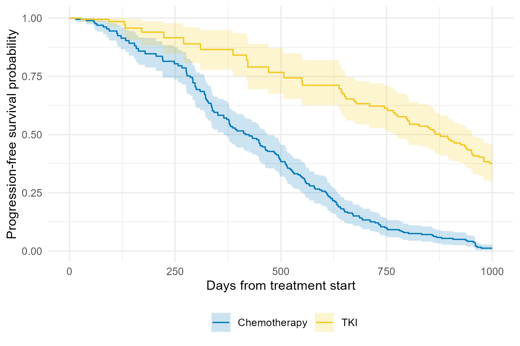

Patients in the TKI group have higher progression-free survival probability than those in the chemotherapy group, and that the bootstrap-based confidence intervals are not overlapping for most of the follow-up period.

IPCW Cox regression

Next, estimate the hazard ratio (HR) for the association between treatment group and PFS, accounting for the dependent censoring.

Use the convenience wrapper get_ipcw_cox_fit_se() to obtain a tibble of results from the weighted Cox regression model.

cox_fit <- get_ipcw_cox_fit_se(dat_long, weight = "wgt")

cox_fit
#> # A tibble: 1 × 7
#>   term  log_hr log_hr_se log_hr_rob_se    hr hr_ci_low hr_ci_high
#>   <chr>  <dbl>     <dbl>         <dbl> <dbl>     <dbl>      <dbl>
#> 1 x      -1.41     0.109         0.183 0.243     0.170      0.348

Then fit the Cox model to each of the bootstrap datasets and extract the log(HR) from each model fit. These will be used to construct bootstrap percentile intervals. Because this process takes some time, the resulting object cox_boot_lhr is included in this package.

# Fit the Cox model to the B bootstrap samples
cox_boot_fit <-
  boot_dat |>
  map(~ get_ipcw_cox_fit_se(., covariate = "x", weight = "wgt"))

# Extract the B log HRs 
cox_boot_lhr <- 
  map_dbl(cox_boot_fit, "log_hr")

Use the function get_boot_pci_se() on a dataframe of the log(HR)s to obtain the bootstrap-based 95% confidence interval.

# Calculate the bootstrap percentile interval
boot_pci <- get_boot_pci_se(data.frame(log_hr = cox_boot_lhr))

And combine the results into a table:

result_tab <- data.frame(
  Scale = c("log(HR)", "HR"),
  Estimate = round(c(cox_fit$log_hr, exp(cox_fit$log_hr)), 2),
  Lower_95pct_PI = round(c(boot_pci[[1]], exp(boot_pci[[1]])), 2),
  Upper_95pct_PI = round(c(boot_pci[[2]], exp(boot_pci[[2]])), 2)
)

result_tab |> 
  gt() |> 
  cols_label(
    Scale = "Scale",
    Estimate = "Estimate",
    Lower_95pct_PI = "Lower 95% PI",
    Upper_95pct_PI = "Upper 95% PI"
  ) |> 
  # Add a footnote
  tab_footnote(
    footnote = "PI = percentile interval",
    locations = cells_column_labels(columns = c(Lower_95pct_PI, Upper_95pct_PI))
  ) |> 
  tab_header(
    "IPCW Cox regression results for the association between treatment group and progression-free survival"
  )

Scale	Estimate	Lower 95% PI¹	Upper 95% PI¹
IPCW Cox regression results for the association between treatment group and progression-free survival
log(HR)	-1.41	-1.55	-0.95
HR	0.24	0.21	0.39
¹ PI = percentile interval