ppseq
The {ppseq} package provides functions to design clinical trials using Bayesian sequential predictive probability monitoring. Functionality is available to design one-arm or two-arm trials by searching over a grid of combinations of posterior and predictive thresholds and identifying the optimal design according to two criteria: accuracy and efficiency. Interactive plotting allows easy comparison of the various design options and easy trial implementation through decision rule plots.
Installation
You can install the production version of ppseq from CRAN with:
install.packages("ppseq")Or you can install the development version of ppseq from GitHub with:
remotes::install_github("zabore/ppseq")Basic usage
The primary function to search over a grid of combinations of posterior and predictive thresholds for a certain trial design is calibrate_thresholds(). This function is computationally intensive to varying degrees depending on the number of looks and the number of threshold combinations, and is best run on a server and/or with parallelization.
set.seed(12345)

calthresh <-
  calibrate_thresholds(
    p_null = c(0.2, 0.2),
    p_alt = c(0.2, 0.5),
    n = cbind(seq(10, 50, 10), seq(10, 50, 10)),
    N = c(50, 50),
    pp_threshold = seq(0.9, 0.95, 0.01),
    ppp_threshold = seq(0.05, 0.2, 0.05),
    delta = 0
    )
The resulting design options can be compared interactively compared by passing the results to plot() with the option plotly = TRUE. Static versions of the plots are also available using the default option plotly = FALSE, which produces ggplot results. Plot output can optionally be filtered by desired range of type 1 error and minimum power. The default plots all design options. The results can also be viewed in tabular form by passing the results to print() with filtering options for the desired range of type 1 error and minimum power.
plot(calthresh)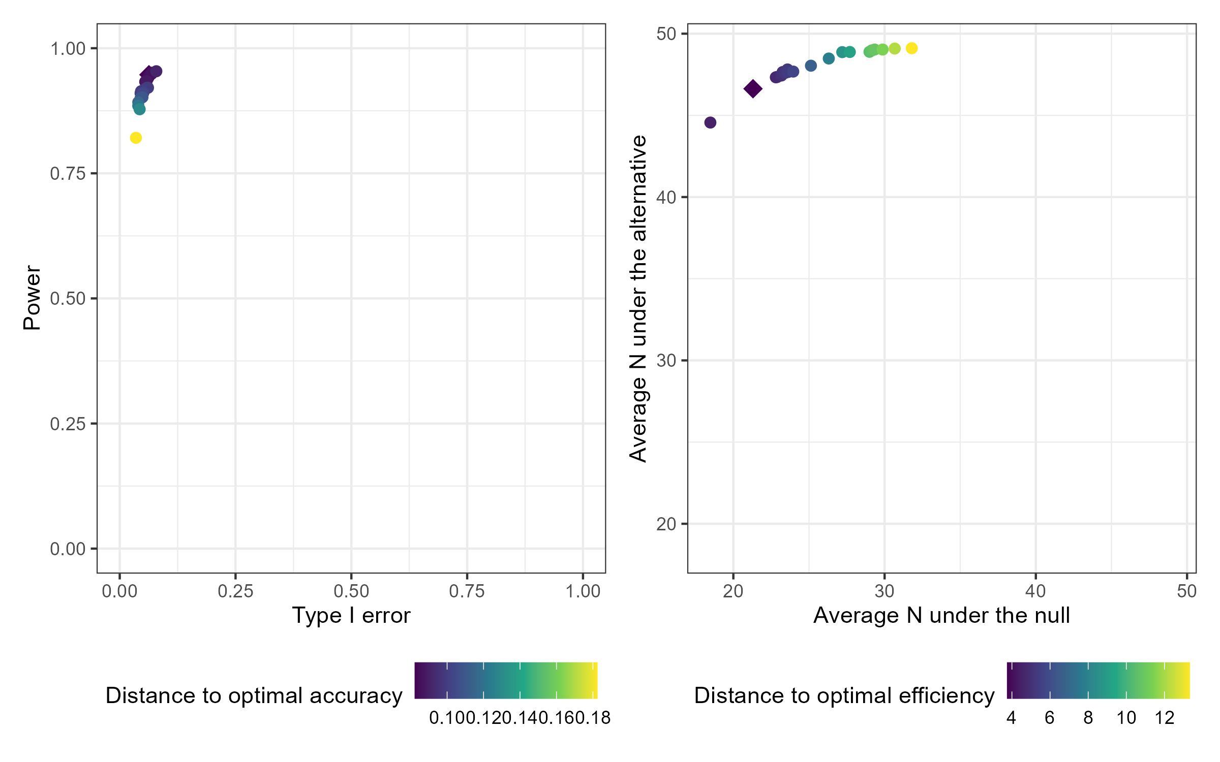
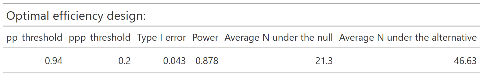
The optimal accuracy and optimal efficiency designs can be obtained by passing the results to the optimize_design() function, with filtering applied for the desired range of type 1 error and minimum power.
optimize_design(calthresh, type1_range = c(0.025, 0.05), minimum_power = 0.8)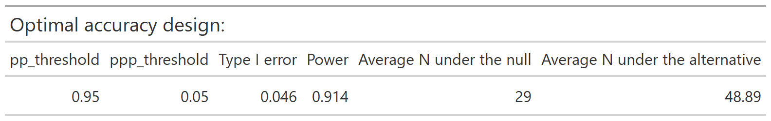
After selecting a design, we can obtain a set of decision rules to implement the trial, so that no calculations will be needed during the course of the trial. The calc_decision_rules() function will generate the decision rules to stop or continue at each interim look of the trial.
set.seed(123456)

opteffrules <-
  calc_decision_rules(
    n = cbind(seq(10, 50, 10), seq(10, 50, 10)),
    N = c(50, 50),
    theta = 0.94,
    ppp = 0.2,
    p0 = NULL,
    delta = 0
  )
The results can be displayed with interactive graphics by passing the results to plot() with the default option plotly = TRUE. Below are the static ggplot versions created with the option plotly = FALSE for demonstration purposes. Tabular results can be obtained by passing the results to print().
plot(opteffrules, plotly = FALSE)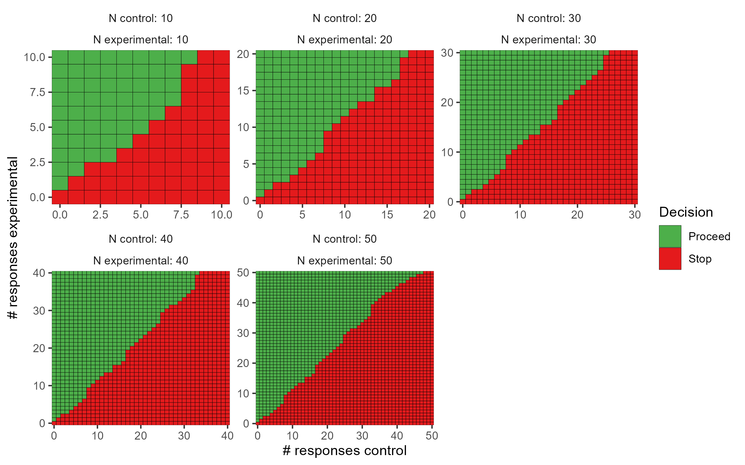
See the vignettes for the one-sample and two-sample cases for additional details about available features and options.