condsurv

The condsurv package contains a function for generating conditional survival estimates with associated confidence intervals, and a function for plotting conditional survival curves.

Installation

Install the package using

pak::pak("zabore/condsurv")

Estimate conditional survival

library(condsurv)
library(dplyr)
library(survival)

If $S(t)$ represents the survival function at time $t$, then conditional survival is defined as

$$S(y|x) = \frac{S(x + y)}{S(x)}$$

where $y$ is the number of additional survival years of interest and $x$ is the number of years a subject has already survived.

The conditional_surv_est function will generate this estimate along with 95% confidence intervals.

The lung dataset from the survival package will be used to illustrate.

# Scale the time variable to be in years rather than days
lung2 <- 
  mutate(
    lung,
    os_yrs = time / 365.25
  )

First generate a single conditional survival estimate. This is the conditional survival of surviving to 1 year conditioned on already having survived 6 months ($0.5$ year). This returns a list, where cs_est is the conditional survival estimate, cs_lci is the lower bound of the 95% confidence interval and cs_uci is the upper bound of the 95% confidence interval.

myfit <- survfit(Surv(os_yrs, status) ~ 1, data = lung2)

conditional_surv_est(
  basekm = myfit,
  t1 = 0.5, 
  t2 = 1
)
#> $cs_est
#> [1] 0.58
#> 
#> $cs_lci
#> [1] 0.49
#> 
#> $cs_uci
#> [1] 0.66

You can easily use purrr::map_df to get a table of estimates for multiple timepoints. For example we could get the conditional survival estimate of surviving to a variety of different time points given that the subject has already survived for 6 months (0.5 years).

prob_times <- seq(1, 2.5, 0.5)

purrr::map_df(
  prob_times, 
  ~conditional_surv_est(
    basekm = myfit, 
    t1 = 0.5, 
    t2 = .x) 
  ) %>% 
  dplyr::mutate(years = prob_times) %>% 
  dplyr::select(years, everything()) %>% 
  knitr::kable()

years	cs_est	cs_lci	cs_uci
1.0	0.58	0.49	0.66
1.5	0.36	0.27	0.45
2.0	0.16	0.10	0.25
2.5	0.07	0.02	0.15

A note on confidence interval estimation

The confidence intervals are based on a variation of the log-log transformation, also known as the “exponential” Greenwood formula, where the conditional survival estimate is substituted in for the traditional survival estimate in constructing the confidence interval.

If $\hat{S}(y|x)$ is the estimated conditional survival to $y$ given having already survived to $x$, then

$$\hat{S}(y|x)^{exp(\pm1.96\sqrt{\hat{L}(y|x)})}$$

where

$$\hat{L}(y|x)=\frac{1}{\log(\hat{S}(y|x))^2}\sum_{j:x \leq \tau_j \leq y}\frac{d_j}{(r_j-d_j)r_j}$$

and

$\tau_j$ = distinct death time $j$

$d_j$ = number of failures at death time $j$

$r_j$ = number at risk at death time $j$

Plot conditional survival curves

library(ggplot2)

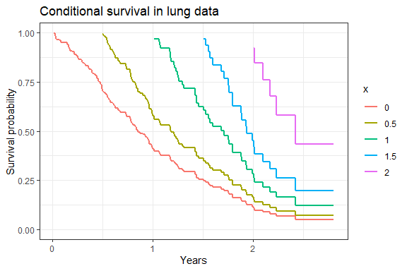
To plot the conditional survival curves at baseline, and for those who have survived 6 months, 1 year, 1.5 years, and 2 years, we use the gg_conditional_surv function.

The lung dataset from the survival package will be used to illustrate.

# Scale the time variable to be in years rather than days
lung2 <- 
  mutate(
    lung,
    os_yrs = time / 365.25
  )

myfit <- survfit(Surv(os_yrs, status) ~ 1, data = lung2)

cond_times <- seq(0, 2, 0.5)

gg_conditional_surv(
  basekm = myfit, 
  at = cond_times,
  main = "Conditional survival in lung data"
  ) 

Documentation

This package is documented using pkgdown, and the resulting website is available at http://www.emilyzabor.com/condsurv/, where detailed Tutorials can be found covering all of the package functionality.

See http://www.emilyzabor.com/condsurv/reference/ for detailed function documentation.